Suitability and Impact Modeling using Raster Analysis

Goals and Objectives

In this final portion of our case study on Frac Sand mining in western Wisconsin, we wanted to determine what areas within our subset of the southern portion of Trempealeau County would be best for sand mining. To do this we needed to take into consideration the suitability of the land as well as the impact that a mine would have on a given area. To do this we used a number of different raster layers including DEM (digital elevation model), land use/land cover datasets, geology and more. In order to determine the impact of a mine on a given area we implemented reclassification and euclidean distance tools to understand the impact that a mine would have on vector features like streams, residential areas etc. By creating two separate models, one for suitability and another for impact analysis we were then able to use the raster calculator in order to combine these results and ultimately determine a location index. This index would then give us a spatial representation of the best areas where sand mines should be created to minimize the impact on an area as well as be actually suitable for mining. 

Methods

Suitability Model

To determine the areas which were most suitable for mining we took into consideration 5 different variables:
1. Geology 
2. Land Cover Type
3. Proximity to Rail Terminals
4. Slope of the Area
5. Water Table Depth

Some of these variables were vector features and needed to first be transformed into rasters. In order to determine the most suitable portions of these layers we needed to rank them. Based on this we developed a scale of 1-3 to rank certain areas based on their suitability for mining. The ranking of 1 was given to low suitability while the ranking of 3 was given to the most suitable in most cases (Fig. 1). 

(Fig. 1) This tables explains why and how the suitability rankings were determined.

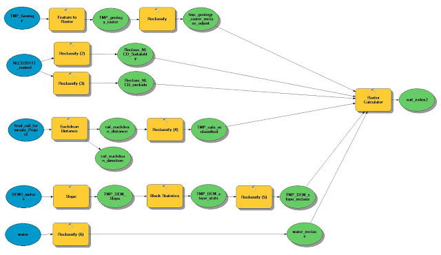
Some cases required an extra step prior to ranking the raster values. For instance, the geology layer we used was originally a vector data set and needed to be changed into a raster using the "feature to raster" tool. The DEM dataset we used we needed to first calculate the slope of an area before ranking the values to make sure we weren't just ranking the elevation values but the slope of certain areas. We also calculated the euclidean distance around rail terminals so we could rank the output based on distance from rail terminals. 

In all cases except for geology types and land cover all the layer variables were given a ranking of 1-3. For the geology types the two main geology types we wanted to select from was the Wonewoc and Jorden formations so they were given a ranking of one. The other geology types in this region of Trempealeau County were given a 0 to signify that they are not at all suitable for sand mining. Despite this single exception the other 5 variables were ranked based on this 1-3 scale where 3 was the most suitable type. As for the land cover variables, a 0 value was assigned to a few land cover types which were impossible for a mine to be built on like open water or wetlands. 

To set all these rankings we needed to use the "reclassify" tool (as seen in Fig. 2). This way we could view the output of the reclassification in a very simple way, as either 1, 2, or 3 rather than all unique values. The outputs of each of these reclassifications can be seen in Fig. 3.

(Fig. 2) Workflow model used to determine the suitability of an area for sand mining. 

(Fig. 3) Maps showing the output of our analysis of each of the 5 variables we took into consideration.

Impact Model

To better understand the areas which would be impacted most if a mine were to be placed in a particular area we looked at the proximity to 5 variables:
1. Farmland
2. Streams
3. Residential Areas
4. Schools
5. Wildlife Areas

(Fig. 4) Workflow model used to determine the impact a sand mine would have on an area.

(Fig. 5) This table shows how and why the rankings were developed for the impact model.

(Fig. 6) Maps showing the output of our analysis of each of the 5 variables we took into consideration.

Suitability and Impact Index

To combine the outputs of both the suitability and impact models we used the "raster calculator" tool to add them together. 

(Fig. 7) This model shows the addition of the output of the suitability and impact models.

Results

Fig. 8

Fig. 9

Discussion / Conclusion

As can be seen in Fig. 9, the areas which are the closest to orange are those which are the most optimal locations for sand mines which maximize suitability and minimize the impact on an area. Ideally only the red areas would be considered for mine locations, but this map helps developers to better understand the areas which should be most avoided in the case of sand mine development. 

It is interesting to think about how easily the reclassifications can impact the overall results of the sustainability and impact models would change. Simply adjusting the values used in the rankings could drastically change the overall output.

Sources

Bureau of Transportation Statistics. (n.d.). Rail terminals feature class. Retrieved December 6, 2015, from http://www.rita.dot.gov/bts/sites/rita.dot.gov.bts/files/subject_areas/geographic_information_services/index.html 

Land Records. (n.d.). Trempealeau County Land Records. Geodatabase. Retrieved December 6, 2015, from http://www.tremplocounty.com/landrecords/ 

United States Geological Survey, National Map Viewer. National Land Cover Database (NLCD) raster and DEM. (n.d). Retrieved December 6, 2015, from http://nationalmap.gov/viewer.html

Wisconsin Geological and Natural History Survey (GNHS). Water table contours. GIS data. (n.d). Retrieved December 6, 2015, from http://wgnhs.uwex.edu/map-data/gis-data/

Wisconsin Geological and Natural History Survey (WGNHS). B.A. Brown, 1988. Bedrock Geology of Wisconsin, West-Central Sheet, WGNHS Map 104. Digitizing by Beatriz Vidru Linhares, University of Wisconsin Eau Claire (UWEC). Retrieved from UWEC GIS resources.

Sand Mining: Network Analysis

Goals and Objectives

The goal of this lab was to use network analysis in ArcMap along with model builder to continue our study of the impacts of frac sand mining in Western Wisconsin. Mines have a wide variety of ways in which they transport their sand including air, rail, truck and usually a combination of two or all these methods. Almost all the sand mined in the Wisconsin is transported out of the state by rail and many companies have begun creating their own railways to speed up the transportation process. Those who do not have a rail system though require the use of public roads to move their sand to the nearest rail depot. Using the Python Script #2, we were able to separate the mines who use trucks to transport their sand to rail facilities to gain a better understanding of the impact that the transportation of this sand has on the public roadways.

Through the use of ArcMap’s model builder and network analysis tool we were able to determine the most likely paths that trucks would be traveling in order to go from the mining site to the closest rail facility. Since these trucks are traveling to and from the mine site to these rail stations they are have an impact on the public road ways, but to what extent we do not know. To understand this in monetary terms we will use a hypothetical value of 2.2 cents per mile to calculate the cost of added maintenance on the roads where sand transportation is prevalent by county. In addition to this we will be making the assumption that each mine takes about 50 trips to the rail facility which is also a hypothetical, arbitrary number. Through the use of model builder and the network analysis tool we will gain a better understanding of how much damage these trucks are having on public roads.

Methods

We used the mine data we produced using Python Script 2. This sorted the original data we received by the Wisconsin DNR and selected the mines which are most likely to have the greatest impact on public roadways. 

To begin the network analysis I used the mine locations we selected in the previous lab and the streets network dataset from ESRI streetmap provided to us. Next, I used model builder to calculate the cost per county required to repair and maintain the public roadways used by mines to transport sand from the mine to rail facilities (Fig. 1). I started by adding the "Make Closest Facility Layer" tool, making the mines as the incidents and the rail stations as the facilities. I also added the "Add Location" tool to my model in order to set up the network analysis. In order to run the tool and determine the shortest distance between the mines and the rail facilities, I  had to add the "Solve" tool. I did need to take this data and make it into a feature class of the best routes as calculated by the network analysis, to do this I used the "Select Data" and "Copy Features" tools. Since the calculated route was in a geographic coordinate system it needed to be projected, using the "Project" tool, into a projected coordinate system. In this case I used the NAD 1983 HARN Transverse Mercator (feet) in order to allow for the calculations to be accurate. 

To calculate the total amount of distance traveled by trucks I used the "Tabulate Intersection" tool in order to take the Wisconsin county boundaies and computed the overall distance of the routes within each of them. Next I needed to create a new field and within the table to show this distance per county. Then I created another new field where I calculated the cost of the damage to roads by multiplying the distance field by 2.2 cents per mile. The equation I used was: (distance in miles) * 50 * 0.022. The 50 represents the idea that each mile is traveled by the trucks about 50 times a day. 

(Fig. 1) This is the model used to implement the network analysis tools for this exercise.

Results

The route data could then be shown on a map of Wisconsin (Fig. 2). In order to best understand the results of the model we ran previously we brought the data into Microsoft Excel using the table to excel tool in ArcMap. Once this was done I was able to graph the dollar amounts per county (Fig. 3) and apply that information to a map of Wisconsin counties (Fig. 4).

(Fig. 2) This maps shows the most efficient and likely routes taken by mine company trucks from the mining site to the nearest rail facility. 

(Fig. 3) The cost of road damage caused by mines trucking sand on public roads based on an arbitrary value of 2.2 cents per mile is shown in the graph above by county.

(Fig. 4) This map shows the possible cost in damage to roads by mine company transportation by county.

Discussion

I was surprised at the range of cost per county but generally found that the values were a bit lower than I expected. There is certainly room for error since we are making the assumption that the number of trips being 50 per day. A simple change in this value could drastically shift the calculated costs. The routes could also be effected if we tried to incorporate rail facilities outside of Wisconsin as well. 

It would be very interesting to know what the actual cost of average maintenance on public roadways to better understand how these mines effect roads. For instance, most of the cost is in a few counties and a great deal of this is caused from the longer distances which need to be traveled by trucks since there are fewer rail facilities. 

A major issue with this model though is that the network analysis tool simply calculates the most time efficient route from each mine to a rail facilities but that does not mean that the trucks actually travel this path. Therefore there are some problems with this model but it is the best way to predict the routes and therefore understand the most likely impact that they will have on the roads.

Conclusion

The network analysis tool is very versitile and is fairly simple to use in ArcMap. Not only does it utilize street networks to create the most time efficient route but it can be used in a number of other applications. For instance, companies that deliver products can use this technology to determine the best route based on a number of different stops in order to find the most efficient route. This not only helps to minimize transportation costs but also time spent traveling from one stop to another. In this particular case study we are looking at the impact of semi-truck traffic has on the roadways based on the most likely routes they travel. 

Data Normalization, Geocoding and Error Assessment

Goals and Objectives

The goal of this lab exercise was to geocode the locations of all the sand mines in western Wisconsin and compare our individual results with others in the class as well as the actual mine location point data. The raw data we received was from the Wisconsin DNR and was not properly normalized and therefore could not be directly geocoded using ArcGIS software. In order to use properly use this data we needed to navigate the excel spreadsheet of vague data, normalize it, geocode it and compare the resulting data. A more detailed view of this procedure can be seen below (Fig. 1): 

(Fig. 1) This diagram gives a detailed description of the objectives for this lab exercise.

Methods


The first step in processing the mine data we received directly from the DNR was to normalize it. The original excel datasheet was very disorganized, messy and did not have consistent information. To normalize the data we separated the elements that made up the location field into individual fields including: address (or PLSS), city, state, zip code and the unique mine ID number. While some of the mines had complete addresses others had none and only listed the PLSS (Public Land Survey System) which is Wisconsin's land description system. 

After the table was normalized it was brought in to ArcMap and once we logged into ArcGIS Online we enabled the geocoding tool. Since we connected to the ArcGIS server we were able to use the ESRI address database which located most of the normalized address information we had in our spreadsheet. Initially 18 of my addresses of the 21 total were matched leaving only 3 unmatched. If the program was not able to find the mine based on the address we were able to create a new point to match the attributes. We were also able to adjust the locations of the mines in this interface as well. Some of the unmatched points were due to the use of the PLSS information in place of the normal address fields. Trying to determine where the mines are based on the very vague locations given by the PLSS information was difficult though. We used other resources such as Google Earth to locate the mines and narrow down the search in ArcMap. 

Once all of my geocoding was completed I compared my results to two of my fellow students who were tasked with coding the same mines. To do this I first added their shape file with the mine locations they geocoded and opened the attribute table. There I selected the mines based on the unique mine IDs which were the same as mine and created a new feature layer out of them. I also reprojected the two datasets from my peers to a projected coordinate system. This was done in order to convert the units of the data from degrees to meters so when we calculated the distance between our points it would be reported in meters. In addition to my peer's data I compared my geocoding results to the actual mine locations as measured by the Wisconsin DNR as points. The result of tall these datasets can be seen below in Fig. 2. 

(Fig. 2) The yellow data points show the mine locations based on my geolocation and the red represent the actual mine locations. The data created by my peers are shown as blue and purple points. 

The next step was to compare the distance between my data points and the actual mine locations in order to determine how accurate my geocoding was. To do this I used the point distance tool. I did the same with the data from both of my peers as well. (Originally we were meant to compare our data with a total of 4 other students however 2 of the students who shared the same mine points as me submitted their results.) The results of this distance tool can be seen in the results section of this report. 

Results

Based on my results my geocoded mine locations were "off" compared to the actual sites. The output table showing the distances between my mine data points and the real-world locations can be seen in Fig. 3 and are visually represented in map form in Fig. 4. 

(Fig. 3) This table shows the distance between my geocoded mine sites and the actual location of the mines in meters. 

(Fig. 4) This map shows my geocoded mine locations in orange while the actual mine sites are shown in green. Overall this image is showing in a graphically format the accuracy of my geocoding.

Since each individual in the class was given a different list of unique mines to geocode for this assignment but there was a number of individuals  who had overlapping sites. This was intentionally done to ensure that the mine locations could be compared. Fig. 5 and Fig. 6 show the distance between my geocoded mine sites and my two peers. 

(Fig. 5) This table shows the distance between my geocoded mine sites and the geocoded mines of one of my peers in meters. On average we had a distance of 1,900 meters of distance between our points.

(Fig. 6) This table shows the distance between my geocoded mine sites and the geocoded mines of another one of my peers in meters. On average, we had a distance of about 3,500 meters of distance between our points.

Discussion

Overall the accuracy of my geocoded results compared to the actual mine locations was on average, 2,600 meters apart compared to my results with my peers being about 2,700 meters apart. These errors could have been caused by a number of factors. One could have been a feature coding error because the geocoding tool uses the inputted address to estimate an actual location. In some cases there were multiple mine sites in an area and it was difficult to pinpoint the exact location of the main mine location. 

Another error which could have occurred is the field survey measurement error. Since there was a distinct difference between where the survey crew who created the actual mine location dataset recorded the point to represent the mine and where I recorded the mine during the geocoding process. For example, some of the points in the correct location dataset were taken in the middle of the mine site whereas all of my geocoded locations were based on the main entrance/exit from the mine to the nearest roadway.

Attribute data input could have been another factor which influenced the accuracy of my geocoded data. There might have been some error in the process of normalizing the data which was used to geocode the mine locations. Since we were primarily verifying the mine locations based simply on aerial imagery it is very possible that the wrong mine could have been located based on some incorrect attribute data being entered in the normalization process. 

Conclusion

Despite the complicated procedure, this lab taught us just how important geocoding is to spatial analysis. In addition to this it became clear the role which data normalization plays when trying to create a consistent dataset that can be used to create an accurate geographic representation of the data in the form of a feature class. One factor which could have influenced the overall accuracy of my mine locations compared to the real-world sites is based on where the DNR took the data points in the field. In summary, geocoding is very useful but is not perfect and therefore the results of this method must be used as relative locations. 

Data Gathering and Accuracy Assessment

Goals and Objectives

The goal of this lab exercise was to become more familiar with the process of collecting and downloading data from a variety of different websites and organizations. We then needed to import the data into ArcGIS, join it and project it form different sources into a single, common coordinate system as well as design a geodatabase which can store the data. The main challenge of this lab was to keep all of the downloaded data properly organized and utilize coding methods in the program Python to accelerate the processing step. 

The output data of this lab will be used later in the overall project for this course which is to build a suitability and risk model for sand mining in the western region of the state of Wisconsin. Since our study will focus on Trempealeau County we subsetted the data we downloaded based on this county boundary. This way we can use the specific data just for our area of interest as well as minimize the amount of data we are storing to only what we require. 

Methods

The basic data flow model for this exercise can be seen below: 

The first step in this process was to obtain our data. The sources varied as can be seen below:

• USGS: DEM/Elevation Data
• http://nationalmap.gov/viewers.html
• Trempealeau County Land Records: Trempealeau County Geodatabase
• http://tremplocounty.com/landrecords/
• USDA NRCS Soil Survey: Soils Data
• http://websoilsurvey.sc.egov.usda.gov/App/HomePage.htm
• USDA / NLCD: National Land Use/Land Cover Data
• http://datagateway.nrcs.usda.gov/
• US Department of Transportation: Railroads
• http://rita.dot.gov/bts/sites/ridta.dot.gov.bts/files/publications/national_transportation_atlas_database/2013/index.html

Once all the datasets were downloaded and unzipped into a working folder. Next, we determined which files were the rasters for the DEM, soils information, railroad vector feature class and land use/land cover data and separated these four sets of data into another folder. This data was then used in the next step which was processing the data altogether using Python coding. The coding process itself can be found here.

After all the data was finished being reprojected to the same coordinate system as the rest of the data in the Trempealeau County Geodatabase (NAD83 HARN WISCRS Trempealeau County Feet), was clipped the county boundary and loaded into the geodatabase we were able to access it. It was also crucial to limit the amount of storage space we were using to store unused data so we deleted all redundant data that we downloaded when unzipping the data from the above sources. After all the data was contained in a single geodatabase we were able to create various maps showing the USGS DEM, Land Use/Land Cover, Soil Drainage Index, Railroads and Cropland data for our area of interest, Trempealeau County (Fig. 1).

(Fig. 1) The following data was produced as a result of the Python script we created in order to process the data in a loop form rather than individual images.

Data Accuracy

It is important to determine the accuracy of the data which is used in projects, especially when data used in a single product comes from different sources. Searching through the metadata can help us to better understand where the data comes from, who has had access to it in the past, how frequently it is updated,  the scale etc. In the table below (Fig. 2) the data collected in this lab is organized in a table for each dataset. 

(Fig. 2) The data quality table above was created based on the individual metadata for each dataset. Some of the data was not available in the metadata and hence is represented by the "NA" label.

Conclusion

Being able to properly download and organize data from a variety of sources is critical in the field of geography no matter what specialty. It's also very important to understand the qualities of the data by looking at things like the attribute accuracy, lineage, temporal accuracy etc. The data which we processed using the Python script in this lab will prove to be very useful in our future work on sand mining in western Wisconsin over the course of the semester. 

Sand Mining in Western Wisconsin: An Overview

Despite becoming highly publicized in the last few years, sand mining has been occurring in the state of Wisconsin for over 100 years. In recent years though it has become increasingly popular for its use in the petroleum industry in a process called hydrofracking. Hydrofracking is a method of extracting natural gas and crude oil from rock across the country. Wisconsin contains quality frac sand, or silica sand, however mining for it has other environmental implications. 

Frac sand is in high demand because of its unique grain shape and size which then is suspended in a fluid substance which is then injected into the ground at high pressure into gas and oil wells. The high pressure of the fluid then enlarges fractures in the rock and opens them up to release natural gas and oil trapped within the rock where the wells cannot get to. 

(Fig. 1) Mining process using frac sand and horizontal drilling techniques.

Not all silica sands are used in the process of hydrofracking because the industry specifications are so specific. For instance, the frac sand needs to be almost purely quartz, well rounded and be very strong against compression (Fig. 2).  The major areas which this sand can be found are in regions of western Wisconsin including Burnett and Chippewa Counties, as well as Trempealeau, Jackson and Monroe counties.

(Fig. 2) This image shows frac sand and is shown to scale alongside a dime.

There are typically about seven stages in the process of the frac sand mining operation which include: overburden removal, excavation, blasting, crushing, processing, transportation and reclamation.Before the actual mining begins the overburden must be removed from the top of the sand formation at the site. Overburden is the portion of the soil which is not desired and must be removed prior to extraction of the frac sand product. Next, excavation and blasting begins in order to break apart the very heavily cemented sandstone. During this process locals can be disrupted by the noise and dust. Once the blasting is done the larger blocks of sandstone are moved to another site and broken into smaller grains. These grains are then processed into a uniform size. The processed frac sand is then transported to facturing sites around the country. There are extensive regulations depending on the location.

(Fig. 3) Locations of frac sand mines in the state of Wisconsin are represented by the red squares, while the sandstone formations are shown in gold.

Throughout this course we will be exploring the various controversial issues concerning frac sand mining. It is important to understand the risk of sand mining in western Wisconsin and sustainability. While frac sand mining can really boost local economy it can also have negative effects on the environment. These mining operations offer jobs for locals there have also been links to causing negative health effects to employees and locals because of the dust produced during the mining process. By the end of the semester we hope to have a better idea of how to incorporate sustainable practices throughout the known mines in Wisconsin. 

Sources

• http://wcwrpc.org/frac-sand-factsheet.pdf 
• http://dnr.wi.gov/topic/Mines/documents/SilicaSandMiningFinal.pdf 
• http://www.propublica.org/special/hydraulic-fracturing-national
• http://wisconsinsand.org/assets/downloads/Econ-Impact-in-Wood-County.pdf